Environmental Data

Mattia Rossi

2019-10-04

Connect to MonalisR

First of all we have to load the MonalisR package

library(MonalisR)
library(tibble)

Then we have to Set the path to the Database we want to access. If this field is left empty the URL is automatically set to the MONALISA Database

# Set the Path to the SOS JSON
SOS<-setMonalisaURL() # The Default Path for this Function is already the MONALISA Database
SOS

## [1] "http://monalisasos.eurac.edu/sos/api/v1/timeseries/"

Explore the Database

Once connected to the database we can access the single entries by specifying single subsets in th getMonalisaDB function. We’ve already implemented some functionalities to deal with the data entries

1. First of all we can extract the complete dataset from the Database. This is the most commonly used approach to get a broad overview available data within the database

mnls_all<-getMonalisaDB(url=SOS,subset = "all")
mnls_all<-as_tibble(mnls_all)
print(mnls_all)

## # A tibble: 353 x 4
##    id    label uom   station$propert~ $$label $geometry$coord~ $$type $type
##    <chr> <chr> <chr>            <int> <chr>   <list>           <chr>  <chr>
##  1 2060  Air ~ MHzg               220 Laimbu~ <dbl [3]>        Point  Feat~
##  2 1972  Air ~ %                  211 Algund2 <dbl [3]>        Point  Feat~
##  3 1772  Air ~ %                  193 Girlan~ <dbl [3]>        Point  Feat~
##  4 1978  Air ~ %                  212 Gries2~ <dbl [3]>        Point  Feat~
##  5 1984  Air ~ %                  213 Lana6   <dbl [3]>        Point  Feat~
##  6 1760  Air ~ %                  191 Nals2O~ <dbl [3]>        Point  Feat~
##  7 1766  Air ~ %                  192 Neumar~ <dbl [3]>        Point  Feat~
##  8 1990  Air ~ %                  214 Terlan3 <dbl [3]>        Point  Feat~
##  9 1784  Air ~ %                  195 Terlan~ <dbl [3]>        Point  Feat~
## 10 1996  Air ~ %                  215 Tramin~ <dbl [3]>        Point  Feat~
## # ... with 343 more rows

2. We can extract only the FOIs, Procedures and Properties together with the central ID of each data entry

# Get the list of FOIs
mnls_foi<-getMonalisaDB(url=SOS,subset = "foi")
str(mnls_foi)

##  chr [1:31] "LaimburgProvince" "Algund2" "Girlan1Lamm" ...

# Get the list of properties
mnls_props<-getMonalisaDB(url=SOS,subset = "property")
str(mnls_props)

##  chr [1:76] "Air Humidity - 10 minute average" ...

# Get the list of procedures
mnls_proc<-getMonalisaDB(url=SOS,subset = "procedure")
str(mnls_proc)

##  chr [1:74] "MeteoSensors_LaimburgProvince" "MeteoSensors_Algund2" ...

# Get a combined list of available DOI, PRocedures and Propertoes by ID
mnls_comb<-getMonalisaDB(url=SOS,subset = "combined")
mnls_comb<-as_tibble(mnls_comb)
print(mnls_comb)

## # A tibble: 353 x 4
##    id    foi                 proc                       prop               
##    <chr> <chr>               <chr>                      <chr>              
##  1 2060  LaimburgProvince    MeteoSensors_LaimburgProv~ Air Humidity - 10 ~
##  2 1972  Algund2             MeteoSensors_Algund2       Air Humidity - 5 m~
##  3 1772  Girlan1Lamm         MeteoSensors_Girlan1Lamm   Air Humidity - 5 m~
##  4 1978  Gries2NeufeldGreif~ MeteoSensors_Gries2Neufel~ Air Humidity - 5 m~
##  5 1984  Lana6               MeteoSensors_Lana6         Air Humidity - 5 m~
##  6 1760  Nals2OberauCarli    MeteoSensors_Nals2OberauC~ Air Humidity - 5 m~
##  7 1766  NeumarktStiermoos   MeteoSensors_NeumarktStie~ Air Humidity - 5 m~
##  8 1990  Terlan3             MeteoSensors_Terlan3       Air Humidity - 5 m~
##  9 1784  Terlan3a            MeteoSensors_Terlan3a      Air Humidity - 5 m~
## 10 1996  Tramin13er          MeteoSensors_Tramin13er    Air Humidity - 5 m~
## # ... with 343 more rows

3. We can also limit ourselves to interrogate the geometry of the stations available in the database

mnls_geom <- getMonalisaDB(url=SOS,subset = "geom") 
mnls_geom <- as_tibble(mnls_geom)
print(mnls_geom)

## # A tibble: 31 x 3
##    FOI                            LAT       LON      
##    <chr>                          <chr>     <chr>    
##  1 LaimburgProvince               11.288711 46.382457
##  2 Algund2                        11.123873 46.685781
##  3 Girlan1Lamm                    11.279533 46.455895
##  4 Gries2NeufeldGreifensteinerweg 11.280283 46.501757
##  5 Lana6                          11.151788 46.616553
##  6 Nals2OberauCarli               11.205704 46.560132
##  7 NeumarktStiermoos              11.262795 46.304704
##  8 Terlan3                        11.228543 46.541054
##  9 Terlan3a                       11.228615 46.540983
## 10 Tramin13er                     11.244507 46.329177
## # ... with 21 more rows

Download

Now if we want to download the data we can access all of it by specifying the entries we can see with the prior functions to the downloadMonalisa function:

# Download
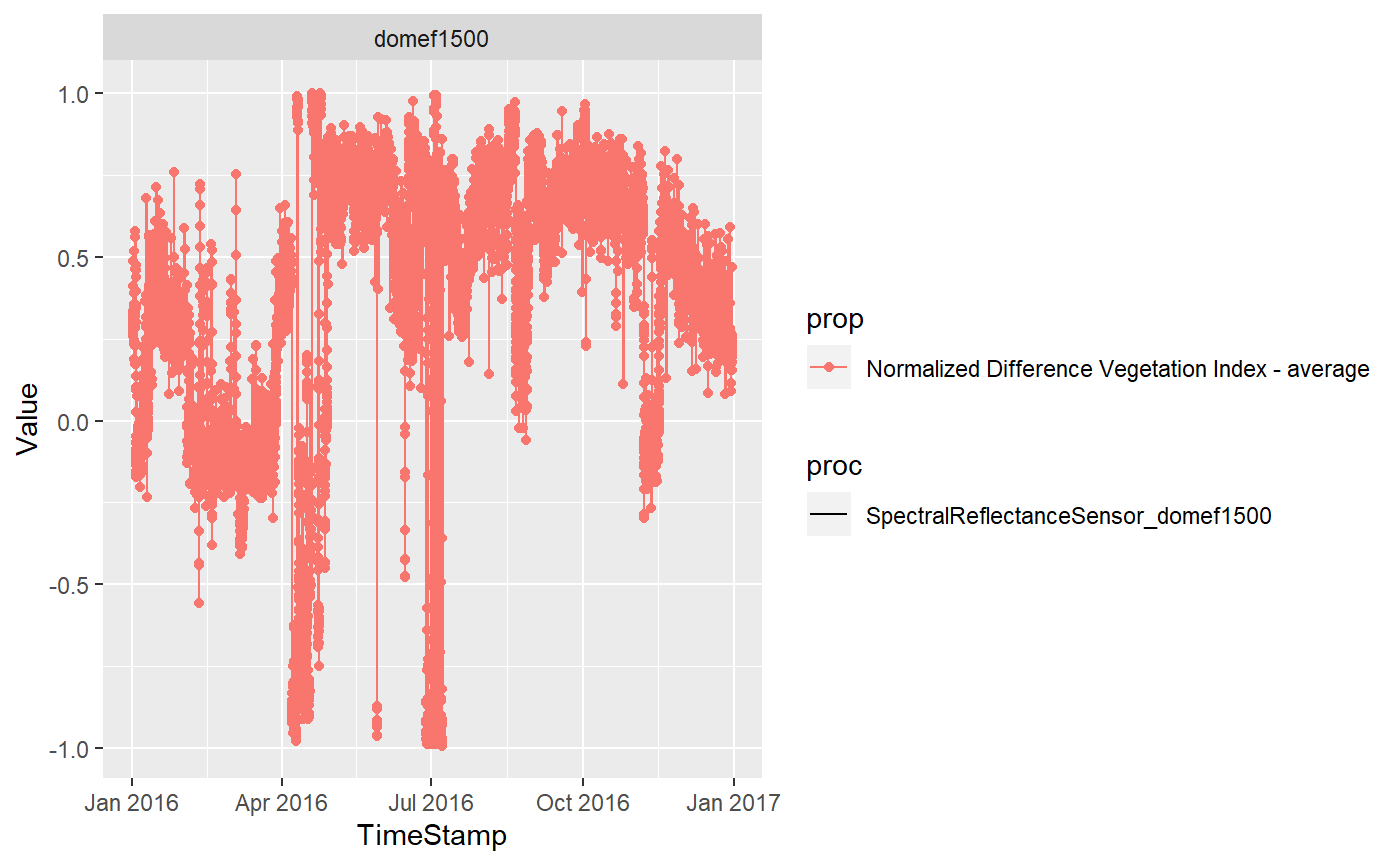
foi1  <-"domef1500"
proc1 <-""
prop1 <-"Normalized Difference Vegetation Index - average"
s <- "2016-01-01 00:00"
e <- "2016-12-31 00:00"

down<-downloadMonalisa(starturl=SOS,datestart=s,dateend=e,foi=foi1,procedure=proc1,property=prop1)
down

## # A tibble: 1 x 5
##   id    foi     proc                 prop                      Data        
##   <fct> <fct>   <fct>                <fct>                     <list>      
## 1 1877  domef1~ SpectralReflectance~ Normalized Difference Ve~ <tibble [17~

The data is stored in “nested tibbles”. One row contains a set of Lists. Use the tidyr::unnest function to enhance the dimensionality and to visualize the complete dataset

library("tidyr")
dat1<-unnest(down)

Plot

For the leaflet graphic we created a simple interface visualizing

plotMonalisaLeaflet()

Simple graphics with GGplots are also easy to produce. The data structure is already in the format proposed within the tidyverse

library("ggplot2")
ggplot(dat1,aes(TimeStamp,Value,col=prop,lty=proc))+geom_line()+geom_point()+facet_wrap(.~foi)